Tag Archives: machine learning

What was Old is New: Finding Joy in Modernising Legacy Systems

(cover image from ThisisEngineering RAEng)

Let’s face it: software is easier to write than maintain. This is why we, as software engineers, prefer to just “rip it out and start over” instead of trying to understand what another developer (or our past self) was thinking. We seem to have collectively forgotten that “programs must be written for people to read, and only incidentally for machines to execute”. You know it’s true — we’ve all had to painstakingly trace through a casserole of spaghetti code and thin, old-world-style abstractions digging for the meat of the program only to find nothing but a mess at the bottom of our plates.

It’s easy to yell “WTF” and blame the previous dev, but the truth is often more complicated. We can’t see the future, so it’s impossible to understand how requirements, technology, or business goals will grow when we design a net-new system. As a result, systems can become unreadable as their scope increases along with the business’s dependency on them. This is a bit of a paradox: older, harder to maintain systems often provide the most value. They are hard to work on because they’ve grown with the company, and scary to work on because breaking it could be a catastrophe.

Here’s where I’m calling you out: if you like hard, rewarding problems… try it. Take the oldest system you have and make it maintainable. You know the one I’m talking about — the one no one will “own”. That one the other departments depend on but engineers hate. The one you had to patch Log4Shell on first. Do it. I dare you.I recently had such an opportunity to update a decade old machine learning system at Bazaarvoice. On the surface, it didn’t sound exciting: this thing didn’t even have neural networks! Who cares! We ll… it mattered. This system processes nearly every user-generated product review received by Bazaarvoice — nearly 9 million per month — and does so with 90 million inference calls to machine learning models. Yup — 90 million inferences! It’s a huge scale, and I couldn’t wait to dive in.

In this post, I’ll share how modernizing this system through a re-architecture, instead of a re-write, allowed us to make it scalable and cost-effective without having to rip out all of the code and start over. The resulting system is serverless, containerized, and maintainable while reducing our hosting costs by nearly 80%. This post is a companion piece to a talk I recently presented at AWS Data Summit for Software Companies on generating value from data by leveraging our best practices to ensure success in machine learning projects. This post discusses the technical aspects in more detail, but you can watch the high-level talk linked at the end.

Something Old

First, let’s take a look at what we’re dealing with here. The legacy system my team was updating moderates user-generated content for all of Bazaarvoice. Specifically, it determines if each piece of content is appropriate for our client’s websites.

Photo by Diane Picchiottino

This sounds straightforward — eliminate obvious infractions such as hate speech, foul language, or solicitations — but in practice, it’s much more nuanced. Each client has unique requirements for what they consider appropriate. Beer brands, for example, would expect discussions of alcohol, but a children’s brand may not. We capture these client-specific options when we onboard new clients, and our Client Services team encodes them into a management database.

For some added complexity, we also sample a subset of our content to be moderated by human moderators. This allows us to continuously measure the performance of our models and discover opportunities for building more models.

The full architecture of our legacy system is shown below:

Our legacy moderation system hosted machine learning models on a single EC2 instance. This made deployments slow and limited scalability to the host’s memory size.

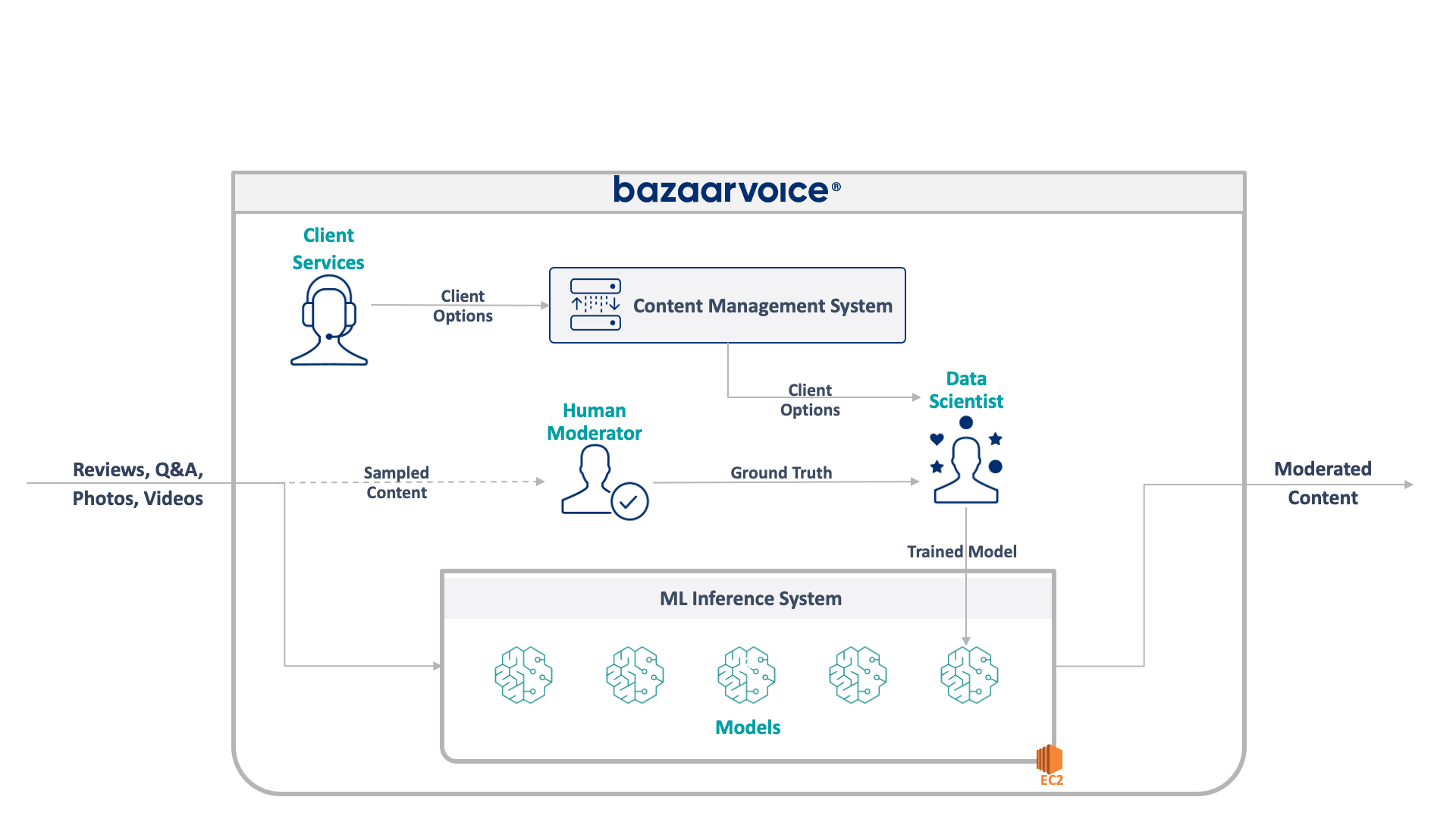
This system has some serious drawbacks. Specifically — all of the models are hosted on a single EC2 instance. This wasn’t due to bad engineering — just the inability of the original programmers to foresee the scale desired by the company. No one thought that it would grow as much as it did. In addition, the system suffered from developer rejection: it was written in Scala, which few engineers understood. Thus, it was often overlooked for improvement since no one wanted to touch it.

As a result, the system continued to grow in a keep-the-lights-on manner. Once we got around to re-architecting it, it was running on a single x1e.8xlarge instance. This thing had nearly a terabyte of ram and costs about $5,000/month (unreserved) to operate. Don’t worry, though, we just launched a second one for redundancy and a third for QA 🙃.

This system was costly to run and was at a high risk of failure (a single bad model can take down the whole service). Furthermore, the code base had not been actively developed and was thus significantly out of date with modern data science packages and did not follow our standard practices for services written in Scala.

Something New

When redesigning this system we had a clear goal: make it scalable. Reducing operating costs was a secondary goal, as was easing model and code management.

The new design we came up with is illustrated below:

Our new architecture deploys each model to a SageMaker Serverless endpoint. This lets us scale the number of models without limit while maintaining a small cost footprint.

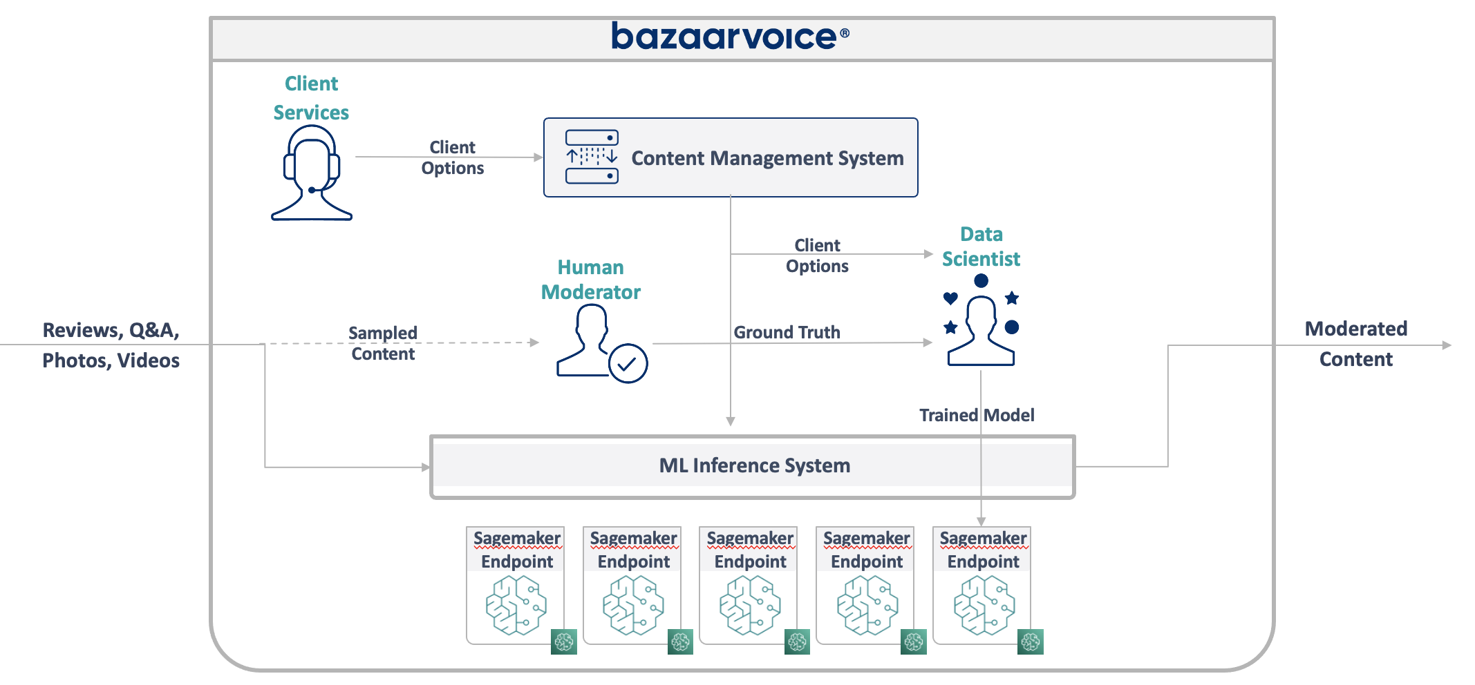
Our approach to solving all of this was to put each machine learning model on an isolated SageMaker Serverless endpoint. Like AWS Lambda functions, serverless endpoints turn off when not in use — saving us runtime costs for infrequently used models. They also can scale out quickly in response to increases in traffic.

In addition, we exposed the client options to a single microservice that routes content to the appropriate models. This was the bulk of the new code we had to write: a small API that was easy to maintain and let our data scientists more easily update and deploy new models.

This approach has the following benefits:

  • Decreased the time to value by over 6x. Specifically, routing traffic to existing models is instantaneous, and deploying new models can be done in under 5 minutes instead of 30.
  • Scale without limit – we currently have 400 models but plan to scale to thousands to continue to increase the amount of content we can automatically moderate.
  • Saw a cost reduction of 82% moving off EC2 as the functions turn off when not in use, and we’re not paying for top-tier machines that are underutilized.

Simply designing an ideal architecture, however, isn’t the really interesting hard part of rebuilding a legacy system — you have to migrate to it.

Something Borrowed

Our first challenge in migration was figuring out how the heck to migrate a Java WEKA model to run on SageMaker, let alone SageMaker Serverless.

Fortunately, SageMaker deploys models in Docker containers, so at least we could freeze the Java and dependency versions to match our old code. This would help ensure the models hosted in the new system returned the same results as the legacy one.

Photo from JJ Ying

To make the container compatible with SageMaker, all you need to do is implement a few specific HTTP endpoints:

  • POST /invocation — accept input, perform inference, and return results.
  • GET /ping — returns 200 if the JVM server is healthy

(We chose to ignore all of the cruft around BYO multimodel containers and the SageMaker inference toolkit.)

A few quick abstractions around com.sun.net.httpserver.HttpServer and we were ready to go.

And you know what? This was actually pretty fun. Toying with Docker containers and forcing something 10 years old into SageMaker Serverless had a bit of a tinkering vibe to it. It was pretty exciting when we got it working — especially when we got the legacy code to build it in our new sbt stack instead of maven. The new sbt stack made it easy to work on, and containerization ensured we could get proper behavior while running in the SageMaker environment.

Something Blue

So we have the models in containers and can deploy them to SageMaker — almost done, right? Not quite.

Photo by Tim Gouw

The hard lesson about migrating to a new architecture is that you must build three times your actual system just to support migration.

In addition to the new system, we had to build:

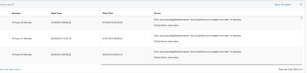
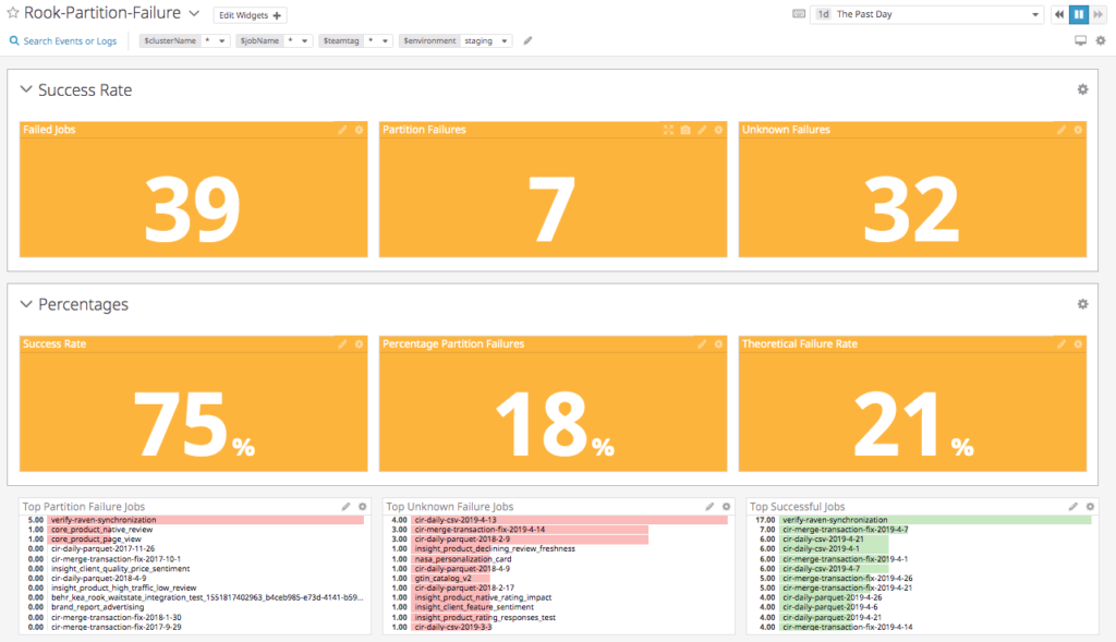
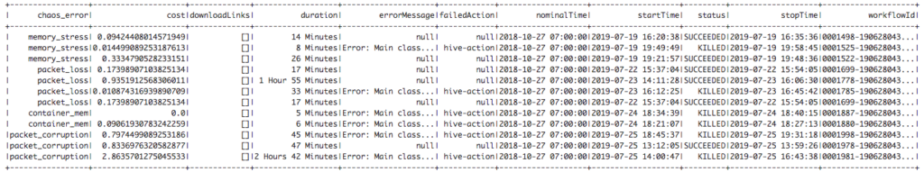
  • A data capture pipeline in the old system to record inputs and outputs from the model. We used these to confirm that the new system would return the same results.
  • A data processing pipeline in the new system to compute results and compare them to the data from the old system. This involved a large amount of measurement with Datadog and needed to offer the ability to replay data when we found discrepancies.
  • A full model deployment system to avoid impacting the users of the old system (which would simply upload models to S3). We knew we wanted to move them to an API eventually, but for the initial release, we needed to do so seamlessly.

All of this was throw-away code we knew we could toss once we finished migrating all of the users, but we still had to build it and ensure that the outputs of the new system matched the old.

Expect this upfront.

While building the migration tools and systems certainly took more than 60% of our engineering time on this project, it too was a fun experience. Unit testing became more like data science experiments: we wrote whole suites to ensure that our output matched exactly. It was a different way of thinking that made the work just that much more fun. A step outside our normal boxes, if you will.

So… Just Try It

Next time you’re tempted to rebuild a system from code up, I’d like to encourage you to try migrating the architecture instead of the code. You’ll find interesting and rewarding technical challenges and will likely enjoy it much more than debugging unexpected edge cases of your new code.


The talk I gave is a bit more high-level and goes into the MLOps side of things. Check it out here:

Kedro 6 Months In

We build AI software in two modes: experimentation and productization. During experimentation, we are trying to see if modern technology will solve our problem. If it does, we move on to productization and build reliable data pipelines at scale.

This presents a cyclical dependency when it comes to data engineering. We need reliable and maintainable data engineering pipelines during experimentation, but don’t know what that pipeline should do until after we’ve completed the experiments. In the past, I and many data scientists I know have used an ad-hoc combination of bash scripts and Jupyter Notebooks to wrangle experimental data. While this may have been the fastest way to get experimental results and model building, it’s really a technical debt that has to be paid down the road.

The Problem

Specifically, the ad-hoc approach to experimental data pipelines causes pain points around:

  • Reproducibility: Ad-hoc experimentation structures puts you at risk of making results that others can’t reproduce, which can lead to product downtime if or when you need to update your approach. Simple mistakes like executing a notebook cell twice or forgetting to seed a random number generator can usually be caught. But other, more insidious problems can occur, such as behavior changes between dependency versions.
  • Readability: If you’ve ever come across another person’s experimental code, you know it’s hard to find where to start. Even documented projects might just say “run x script, y notebook, etc”, and it’s often unclear where the data come from and if you’re on the right track. Similarly, code reviews for data science projects are often hard to read: it’s asking a lot for a reader to differentiate between notebook code for data manipulation and code for visualization.
  • Maintainability: It’s common during data science projects to do some exploratory analysis or generate early results, and then revise how your data is processed or gathered. This becomes difficult and tedious when all of these steps are an unstructured collection of notebooks or scripts. In other words, the pipeline is hard to maintain: updating or changing it requires you to keep track of the whole thing.
  • Shareability: Ad-hoc collections of notebooks and bash scripts are also difficult for a team to work on concurrently. Each member has to ensure their notebooks are up to date (version control on notebooks is less than ideal), and that they have the correct copy of any intermediate data.

Enter Kedro

A lot of the issues above aren’t new to the software engineering discipline and have been largely solved in that space. This is where Kedro comes in. Kedro is a framework for building data engineering pipelines whose structure forces you to follow good software engineering practices. By using Kedro in the experimentation phase of projects, we build maintainable and reproducible data pipelines that produce consistent experimental results.

Specifically, Kedro has you organize your data engineering code into one or more pipelines. Each pipeline consists of a number of nodes: a functional unit that takes some data sets and parameters as inputs and produces new data sets, models, or artifacts.

This simple but strict project structure is augmented by their data catalog: a YAML file that specifies how and where the input and output data sets are to be persisted. The data sets can be stored either locally or in a cloud data storage service such as S3.

I started using Kedro about six months ago, and since then have leveraged it for different experimental data pipelines. Some of these pipelines were for building models that eventually were deployed to production, and some were collaborations with team members. Below, I’ll discuss the good and bad things I’ve found with Kedro and how it helped us create reproducible, maintainable data pipelines.

The Good

  • Reproducibility: I can’t say enough good things here: they nailed it. Their dependency management took a bit of getting used to but it forces a specific version on all dependencies, which is awesome. Also, the ability to just type kedro install and kedro run to execute the whole pipeline is fantastic. You still have to remember to seed random number generators, but even that is easy to remember if you put it in their params.yml file.
  • Function Isolation: Kedro’s fixed project structure encourages you to think about what logical steps are necessary for your pipeline, and write a single node for each step. As a result, each node tends to be short (in terms of lines of code) and specific (in terms of logic). This makes each node easy to write, test, and read later on.
  • Developer Parallelization: The small nodes also make it easier for developers to work together concurrently. It’s easy to spot nodes that won’t depend on each other, and they can be coded concurrently by different people.
  • Intermediate Data: Perhaps my favorite thing about Kedro is the data catalog. Just add the name of an output data set to catalog.yml and BOOM, it’ll be serialized to disk or your cloud data store. This makes it super easy to build up the pipeline: you work on one node, commit it, execute it, and save the results. It also comes in handy when working on a team. I can run an expensive node on a big GPU machine and save the results to S3, and another team member can simply start from there. It’s all baked in.
  • Code Re-usability: I’ll admit I have never re-used a notebook. At best I pulled up an old one to remind myself how I achieved some complex analysis, but even then I had to remember the intricacies of the data. The isolation of nodes, however, makes it easy to re-use them. Also, Kedro’s support for modular pipelines (i.e., packaging a pipeline into a pip package) makes it simple to share common code. We’ve created modular pipelines for common tasks such as image processing.

The Bad

While Kedro has solved many of the quality challenges in experimental data pipelines, we have noticed a few gotchas that required less than elegant work arounds:

  • Incremental Dataset: This support exists for reading data, but it’s lacking for writing datasets. This affected us a few times when we had a node that would take 8-10 hours to run. We lost work if the node failed part of the way through. Similarly, if the result data set didn’t fit in memory, there wasn’t a good way to save incremental results since the writer in Kedro assumes all partitions are in memory. This GitHub issue may fix it if the developers address it, but for now you have to manage partial results on your own.
  • Pipeline Growth: Pipelines can quickly get hard to follow since the input and outputs are just named variables that may or may not exist in the data catalog. Kedro Viz helps with this, but it’s a bit annoying to switch between the navigator and code. We’ve also started enforcing name consistency between the node names and their functions, as well as the data set names in the pipeline and the argument names in the node functions. Finally, making more, smaller pipelines is also a good way to keep your sanity. While all of these techniques help you to mentally keep track, it’s still the trade off you make for coding the pipelines by naming the inputs and outputs.
  • Visualization: This isn’t really considered much in Kedro, and is the one thing I’d say notebooks still have a leg up on. Kedro makes it easy for you to load the Kedro context in a notebook, however, so you can still fire one up to do some visualization. Ultimately, though, I’d love to see better support within Kedro for producing a graphical report that gets persisted to the 08_reporting layer. Right now we worked around this by making a node that renders a notebook to disk, but it’s a hack at best. I’d love better support for generating final, highly visual reports that can be versioned in the data catalog much like the intermediate data.

Conclusion

So am I a Kedro convert? Yah, you betcha. It replaces the spider-web of bash scripts and Python notebooks I used to use for my experimental data pipelines and model training, and enables better collaboration among our teams. It won’t replace a fully productionalized stream-based data pipeline for me, but it absolutely makes sure my experimental pipelines are maintainable, reproducible, and shareable.

Root Cause Analysis for Hadoop Applications

Parth Shah and Thai Bui

Overview

One of the reasons why Hadoop jobs are hard to operate is their inability to provide clear, actionable error diagnostic messages for users. This stems from the fact that Hadoop consists of many interrelated components. When a component fails or behaves poorly, the failure will be cascaded to its dependent components which causes a job to fail.

This blog post is an attempt to help to solve that problem by created a user-friendly, self-serving and actionable Hadoop diagnostic system.

Our Goals

Due to its complex nature, the project was split into multiple components. First, we prototyped a diagnostic tool to help debug Hadoop application failure by providing a clear root cause analysis and save engineering time. Second we purposely inflict failures on a cluster (via a method called chaos testing) and collected the data to understand how certain log messages map to errors. Finally, we examined regular expression as well as natural language processing (NLP) techniques to automatically provide root cause analysis in production.

To document this, we organized the blog in the following sections:

  • Error Message Analytics Portal
    • To provide a quick glance at the known root cause.
  • Datadog Dashboard
    • To calculate failure rates related to the unknown root cause and known root cause.
    • Separate infrastructure failure from a missing data failure (missing partition).
  • Data Access
    • All relevant logs messages from services like Yarn, Oozie, HDFS, hive server, etc. were collected and stored under an S3 bucket with an expiration policy.
  • Chaos Data Generation
    • Using chaos testing, we produced actual errors related to memory, network, etc. This was done to understand relationships between log messages and root cause errors.
    • A service was made to create an efficient and simple way to run chaos tests and collect its corresponding/related log data.
  • Diagnostic Message Classification
    • Due to the simple and repetitive nature of log messages (low in entropy), we built a natural language processing model that classified specific error types of an unknown failure.
    • Tested the model on the chaos data for the specific workload at Bazaarvoice

Error Message Analytics Portal

Bazaarvoice provides an internal portal tool for managing analytics applications by the end-users. The following screenshot demonstrates an example message of a “Job failures due to missing data”. This message is caught by using a simple regular expression of the stack trace. A regular expression works because there is only one way a job could fail due to missing data.


DataDog Dashboard

What is a partition?

Partitioning is a strategy of dividing a table into related parts based on date, components or other categories. Using a partition, it is easy and faster to query a portion of data. However, the partition a job is querying can sometimes not be available which causes a job to fail by our design. The dashboard below calculates metrics and keeps track of jobs that failed due to an unavailable partition.

The dashboard classifies failed jobs as either a partition failure (late/missing data) or an unknown failure (Hadoop application failure). Our diagnostic tool attempts to find the root cause of the unknown failures since a late or missing data is an easy problem to solve. 


Data Access

Since our clusters are powered by Apache Ambari, we leveraged and enhanced Ambari Logsearch Logfeeder to ship logs of relevant services directly to S3 and partitioned the data by as shown in the raw_log of the Directory Tree Diagram below. However, as the dataset got bigger, partitioning was not enough to efficiently query the data. To speed up read performance and to iterate faster, the data was later converted into ORC format.


Convert JSON logs to ORC logs

DROP TABLE IF EXISTS default.temp_table_orc;
CREATE EXTERNAL TABLE default.temp_table_orc (
cluster STRING,
file STRING,
thread_name STRING,
level STRING,
event_count INT,
ip STRING,
type STRING,
...
hour INT,
component STRING
) STORED AS ORC
LOCATION 's3a://<bucket_name>/orc-log/${workflowYear}/${workflowMonth}/${workflowDay}/${workflowHour}/';
INSERT INTO default.temp_table_orc SELECT * FROM bazaar_magpie_rook.rook_log
WHERE year=${workflowYear} AND month=${workflowMonth} AND day=${workflowDay} AND hour=${workflowHour};

Sample Queries for Root Cause Diagnosis

SELECT t1.log_message,
       t1.logtime,
       t1.level,
       t1.type,
       t2.Frequency
FROM
  (SELECT log_message,
          logtime,
          TYPE,
          LEVEL
   FROM
     ( SELECT log_message,
              logtime,
              TYPE,
              LEVEL,
              row_number() over (partition BY log_message
                                 ORDER BY logtime) AS r
      FROM bazaar_magpie_rook.rook_log
      WHERE cluster_name = 'cluster_name'
        AND DAY = 28
        AND MONTH=06
        AND LEVEL = 'ERROR' ) S
   WHERE S.r = 1 ) t1
LEFT JOIN
  (SELECT log_message,
          COUNT(log_message) AS Frequency
   FROM bazaar_magpie_rook.rook_log
   WHERE cluster_name = 'cluster_name'
     AND DAY = 28
     AND MONTH=06
     AND LEVEL = 'ERROR'
   GROUP BY log_message) t2 ON t1.log_message = t2.log_message
WHERE t1.logtime BETWEEN '2019-06-28 13:05:00' AND '2019-06-28 13:30:00'
ORDER BY t1.logtime
LIMIT 400;

SELECT log_message, logtime, type
FROM bazaar_magpie_rook.rook_log WHERE level = 'ERROR' AND type != 'logsearch_feeder' AND logtime BETWEEN '2019-06-24 09:05:00' AND '2019-06-24
12:30:10'
ORDER BY logtime
LIMIT 1000;

SELECT log_message, COUNT(log_message) AS Frequency
FROM  bazaar_magpie_rook.rook_log
WHERE cluster_name = 'dev-blue-3' AND level = 'ERROR' AND logtime BETWEEN '2019-06-27 13:50:00' AND '2019-06-29 14:30:00'
GROUP BY log_message
ORDER BY COUNT(log_message) DESC
LIMIT 10;

Chaos Data Generation

The chaos data generation process makes up a bulk of this project as well is the most important. It stems from the process of chaos testing to experiment on software and infrastructure in order to understand the systems ability to withstand unexpected or turbulent conditions. This concept of testing was first introduced by Netflix in 2011. The following pseudocode explains how it works.

Submit a normal job through an API on a specific cluster

Create a list of IP addresses for all the testable nodes in that cluster (such as the workers nodes).

Once we have all associated nodes, inject failures into them (stress test memory or network)

While the job is not done

    Let the job run

At this point, the job has either failed or succeeded

Stop all stress tests

Gather the job details such as start time, end time, status, and most importantly its associated stress test type (memory, packet_corruption, etc.). 

Store job details and its report in JSON format

Job Report Example

{
"duration":"45 Minutes",
"nominalTime":"2018-10-27 07:00:00",
"cost":0.7974499089253186,
"downloadLinks":[],
"errorMessage":"Error: Main class [org.apache.oozie.action.hadoop.Hive2Main], exit code [2]",
"startTime":"2019-07-25 18:45:37",
"stopTime":"2019-07-25 19:31:18","failedAction":"hive-action",
"chaos_error":"packet_corruption",
"workflowId":"0001998-190628043141230-oozie-oozi-W",
"status":"KILLED"
}

We followed the same process to generate chaos data on different types of injected failures such as:

  • High Memory Utilization on the Host
  • Packet Corruption
  • Packet Loss
  • High Memory Util on a Container

While there are certainly more errors the model is capable of learning and classifying, for the purpose of prototyping we kept the type of failures to 2-3 categories.

Diagnostic Message Classification

In this section, we explore 2 types of error classification methods, a simple regex and supervised learning.

Short Term Solution with Regex

There are many ways to analyze text for different patterns. One of these ways is called Regular Expression Matching (regex). Regex is “special strings representing a pattern to be matched in search operation”. One use of regex is finding a keyword like “partition”. When a job fails due to missing partitions its error message usually looks something like this “Not all partitions are available even after 16 attempts“. The regex for this specific case would look like \W*((?i)partition(?-i))\W* .

A regex log parser could easily be able to identify this error and do what is necessary to fix the problem. However, the power of regex is very limiting when it comes to analyzing complex log messages and stack traces. When we find a new error, we would have to manually hardcode a new regular expression to pattern match the new error type which is very error-prone and tedious in the long run.

Since the Hadoop eco-system includes many components, there are many combinations of log messages that can be produced; a simple regex parser would be difficult to work here because it can not process general similarities between different sentences. This is where natural language processing helps.

Long Term Solution with Supervised Learning

The idea behind this solution is to use natural language processing to process log messages and supervised learning to learn and classify errors. This model should work well with log data vs. normal language due since machine logs are more structured and low in entropy. You can think of entropy as a measure of how unstructured or random a set of data is. The English language tends to have high entropy relative to machine logs due to its sometimes illogical sentence structure. On the other hand, machine-generated log data is very repetitive which makes it easier to model and classify.

Our model required pre-processing of logs which are called tokenization. Tokenization is the process of taking a set of text and breaking it up into its individual words or tokens. Next, the set of tokens were used to model their relationship in high dimensional space using Word2Vec. Word2Vec is a widely popular model used for learning vector representation of words called, “word embeddings” (word2vec). Finally, we use the vector representation to train a simple logistic regression classifier using the chaos data generated earlier. The diagram below shows a similar training processing from Experience Report: Log Mining using Natural Language Processing and Application to Anomaly Detection by Christophe Bertero, Matthieu Roy, Carla Sauvanaud and Gilles Tredan.


In contrast to the diagram above, since we only trained the classifier on error logs, it was not possible to classify a normal system as it should produce no error logs. Instead, we trained the data on different types of stressed systems. Using the dataset generated by chaos testing, we were able to identify the root cause for each of the error message for each failed job. This allowed us to make our training dataset as shown below. We split our dataset into a simple 70% training and 30% for testing.

Subsequently, each log message was tokenized to create a word vector. All the tokens were inputted into a pre-trained word2vec model which mapped out each word in a vector space, creating a word embedding. Each line was represented as a list of vectors and an average of all the vectors in a log message represents the feature vector in high dimensional space. We then inputted each feature vector and its labels into a classification algorithm such as logistic regression or random forest to create a model that could predict the root cause error from a logline. However, since failure often contains multiple error log messages, it would not be logical to simply reach a root cause conclusion from just a single line of the log from a long error log. A simple way to tackle this problem would be to window the log and input the individual lines from the window into the model and output the final error as the most common error outputted by all the lines in a window. This is a very naive way of breaking apart long error log so more research would have to be done to process error logs without losing the valuable insight of their dependent messages.

Below are a few examples of error log messages and their tokenized version.

Example Raw Log

java.lang.RuntimeException: org.apache.thrift.transport.TSaslTransportException: No data or no sasl data in the stream at org.apache.thrift.transport.TSaslServerTransport$Factory.getTransport(TSaslServerTransport.java:219)
    at org.apache.thrift.server.TThreadPoolServer$WorkerProcess.run(TThreadPoolServer.java:269)
    at java.util.concurrent.ThreadPoolExecutor.runWorker(ThreadPoolExecutor.java:1149)
    at java.util.concurrent.ThreadPoolExecutor$Worker.run(ThreadPoolExecutor.java:624)
    at java.lang.Thread.run(Thread.java:748) [?:1.8.0_191] Caused by: org.apache.thrift.transport.TSaslTransportException: No data or no sasl data in the stream at org.apache.thrift.transport.TSaslTransport.open(TSaslTransport.java:328)
    at org.apache.thrift.transport.TSaslServerTransport.open(TSaslServerTransport.java:41) ~[hive-exec-3.1.0.3.1.0.0-78.jar:3.1.0-SNAPSHOT] at org.apache.thrift.transport.TSaslServerTransport$Factory.getTransport(TSaslServerTransport.java:216)

Tokenized Raw Log

[java,lang,RuntimeException,org,apache,thrift,transport,TSaslTransportException,No,data,no,sasl,data,stream,org,apache,thrift,transport,TSaslServerTransport,Factory,getTransport,TSaslServerTransport,java219]
[org,apache,thrift,server,TThreadPoolExecutor,WorkerProcess,run,TThreadPoolServer,java,269]
...

Results

The model accurately predicted the root cause of failed job with 99.3% accuracy in our test dataset. At an initial glance, the metrics calculated on the test data look very promising. However, we still need to evaluate its efficiency in production to get a more accurate picture. The initial success in this proof of concept warrants further experimentation, testing, and investigation for using NLP to classify errors. 

Training Data 70% (Top 20 Rows)

Test Data Results 30% (Top 20 Rows)

Conclusion

In order to implement this tool in production, data engineers will have to automate certain aspects of the data aggregation and model building pipeline

Self Reporting Errors

A machine learning model is only as good as its data. For this tool to be robust and accurate, any time engineers encounter a new error or an error that the model does not know about, they should report their belief of the root cause so the corresponding errors logs get tagged with the specific root cause error. For instance, when a job fails for a similar reason, the model will be able to diagnose and classify its error type. This can be done through a simple API, form, Hive query that takes in the job id and its assumed root_cause. The idea behind is this that by creating a form, we could manual label log messages and errors in case the classifier fails to correctly diagnose the true problem. 

The self-reported error should take the form of the chaos error to ensure the existing pipeline will work.

Automating Chaos Data Generation

The chaos tests should run on a regular basis in order to keep the model up to date. This could be done by creating a Jenkins job that automatically runs on a regular cadence. Often times, running a stress test will make certain nodes to be unhealthy. It causes our automation to be unable to SSH into the nodes again to stop the stress test such as when the stress test is interfering with connectivity to the node (see the error below). This can be solved by creating a time limit for the stress test, so the script does not have to ssh again once the job has finished. In the long run, as the self-reported errors grow, the model should rely on chaos test generated test less. Chaos tests produce logs for very extreme situations which could be not typical for a normal production environment. 

java.lang.RuntimeException: Unable to setup local port forwarding to 10.8.100.144:22
    at com.bazaarvoice.rook.infra.util.remote.Gateway.connect(Gateway.java:103)
    at com.bazaarvoice.rook.infra.regress.yarn.RootCauseTest.kill_memory_stress_test(RootCauseTest.java:174)