Recently, during a holiday lull, I decided to look at another way of modeling event stream data (for the purposes of anomaly detection).

I’ve dabbled with (simplistic) event stream models before but this time I decided to take a deeper look at Twitter’s anomaly detection algorithm [1], which in turn is based (more or less) on a 1990 paper on seasonal-trend decomposition [2].

To round it all off, and because of my own personal preference for on-line algorithms with minimal storage and processing requirements, I decided to blend it all with my favorite on-line fading-window statistics math.  On-line algorithms operate with minimal state and no history, and are good choices for real-time systems or systems with a surplus of information flowing through them (https://en.wikipedia.org/wiki/Online_algorithm)

The Problem

The high-level overview of the problem is this: we have massive amounts of data in the form of web interaction events flowing into our system (half a billion page views on Black Friday, for example), and it would be nice to know when something goes wrong with those event streams. In order to recognize when something is wrong we have to be able to model the event stream to know what is right.

A typical event stream consists of several signal components:  a long-term trend (slow increase or decrease in activity over a long time scale, e.g. year over year), cyclic activity (regular change in behavior over a smaller time scale, e.g. 24 hours), noise (so much noise), and possible events of interest (which can look a lot like noise).

This blog post looks at extracting the basic trend, cycle, and noise components from a signal.

Note: The signals processed in this experiment are based on real historical data, but are not actual, current event counts.

The Benefit

The big payback of having a workable model of your system is that when you compare actual system behavior against expected behavior, you can quickly identify problems — significant spikes or drops in activity, for example.  These could be from DDOS attacks, broken client code, broken infrastructure, and so forth — all of which are better to detect sooner than later.

Having accurate models can also let you synthesize test data in a more realistic manner.

The Basic Model

Trend

A first approximation of modeling the event stream comes in the form of a simple average across the data, hour-by-hour:

The blue line is some fairly well-behaved sample data (events per hour) and the green lines are averages across different time windows. Note how the fastest 1-day average takes on the shape of the event stream but is phase-shifted; it doesn’t give us anything useful to test against. The slowest 21-day average gives us a decent trend line for the data, so if we wanted to do a rough de-trending of the signal we could subtract this mean from the raw signal.  Twitter reported better results using the median value for de-trending but since I’m not planning on de-trending the signal in this exploration, and median calculations don’t fit into my lightweight on-line philosophy, I’m going to stay with the mean as trend.

Cycle

While the fast 1-day average takes on the shape of the signal, it is phase shifted and is not a good model of the signal’s cyclic nature. The STL seasonal-trend technique(see [2]) models the cyclic component of the signal (“seasonal” in the paper, but our “season” is a 24-hour span) by creating multiple averages of the signal, one per cycle sub-series.  What this means for our event data is that there will be one average for event counts from 1:00am, another average for 2:00am, and so forth, for a total of 24 running averages:

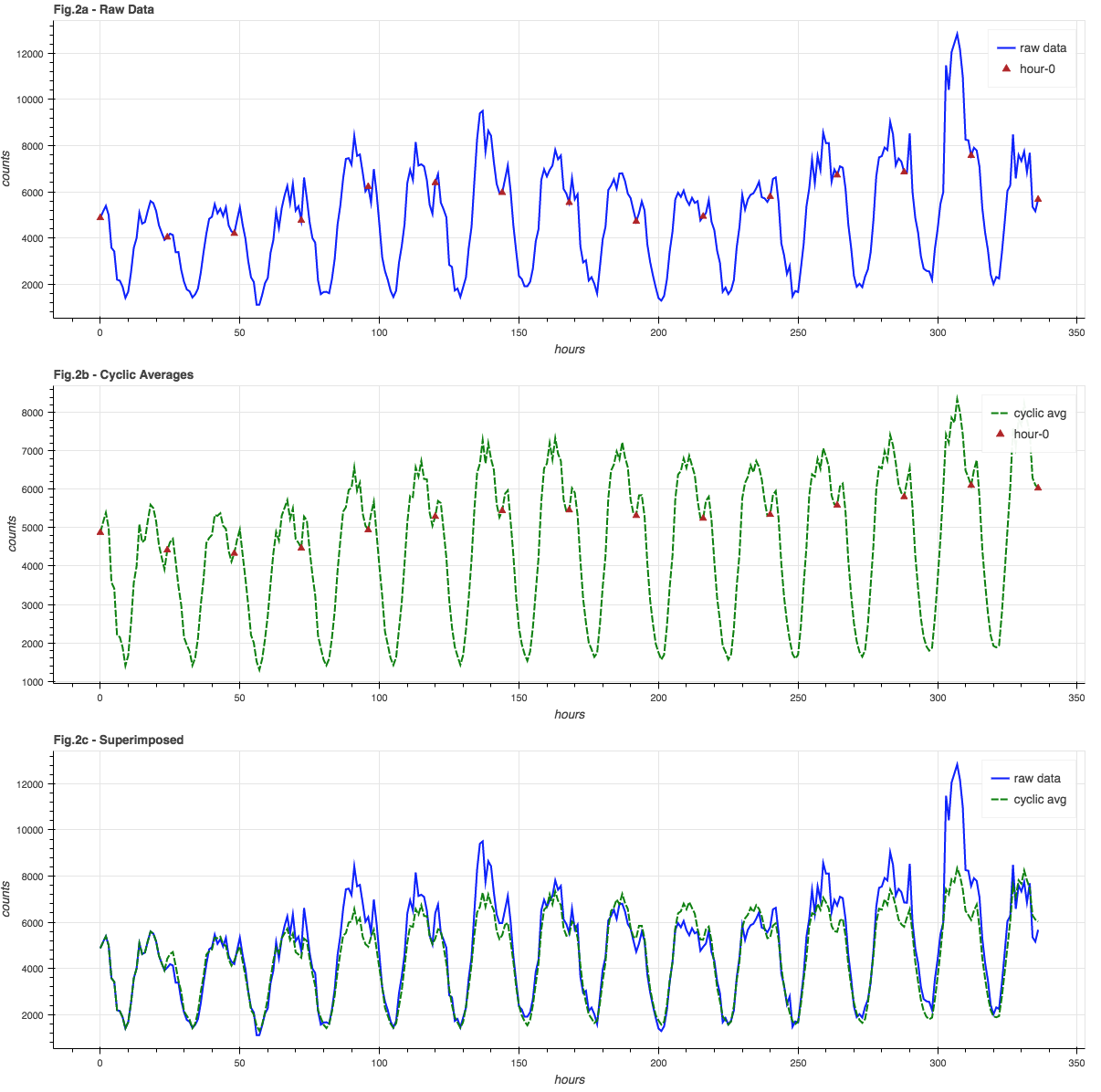
The blue graph in Figure 2a shows the raw data, with red triangles at “hour 0″… these are all averaged together to get the “hour 0” averages in the green graph in Figure 2b.  The green graph is the history of all 24 hourly sub-cycle averages.  It is in-phase with and closely resembles the raw data, which is easier to see in Figure 2c where the signal and cyclic averages are super-imposed.

A side effect of using a moving-window average is that the trend information is automatically incorporated into the cyclic averages, so while we can calculate an overall average, we don’t necessarily need to.

Noise

The noise component is the signal minus the cyclic model and the seasonal trend. Since our online cyclic model incorporates trending already, we can simple subtract the two signals from Figure 2c to give us the noise component, shown in Figure 3:

Some Refinements

Now that we have a basic model in place we can look at some refinements.

Signal Compression

One problem with the basic model is that a huge spike in event counts can unduly distort the underlying cyclic model. A mild version of this can be seen in Figure 4a, where the event spike is clearly reflected in the model after the spike:

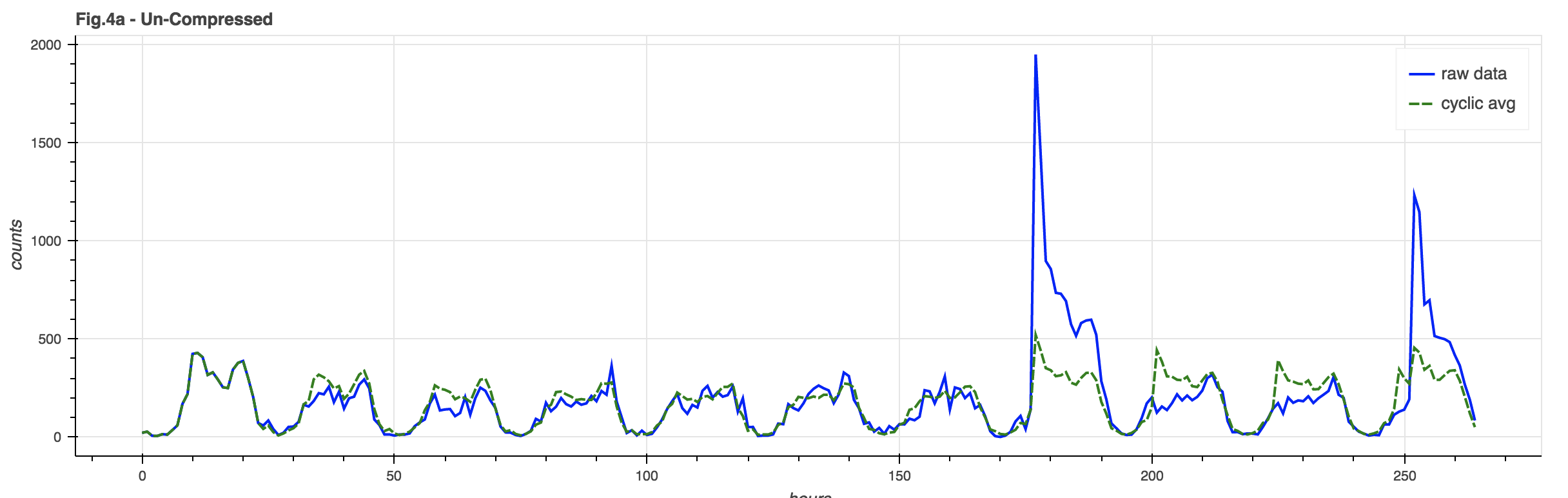
By taking a page out of the audio signal compression handbook, we can squeeze our data to better fit within a “standard of deviation”. There are many different ways to compress a signal, but the one illustrated here is arc-tangent compression that limits the signal to PI/2 times the limit factor (in this case, 4 times the standard deviation of the signal trend):

There is still a spike in the signal but its impact on the cyclic model is greatly reduced, so post-event comparisons are made against a more accurate baseline model.

Event Detection

Now we have a signal, a cyclic model of the signal, and some statistical information about the signal such as its standard deviation along the hourly trend or for each sub-cycle.

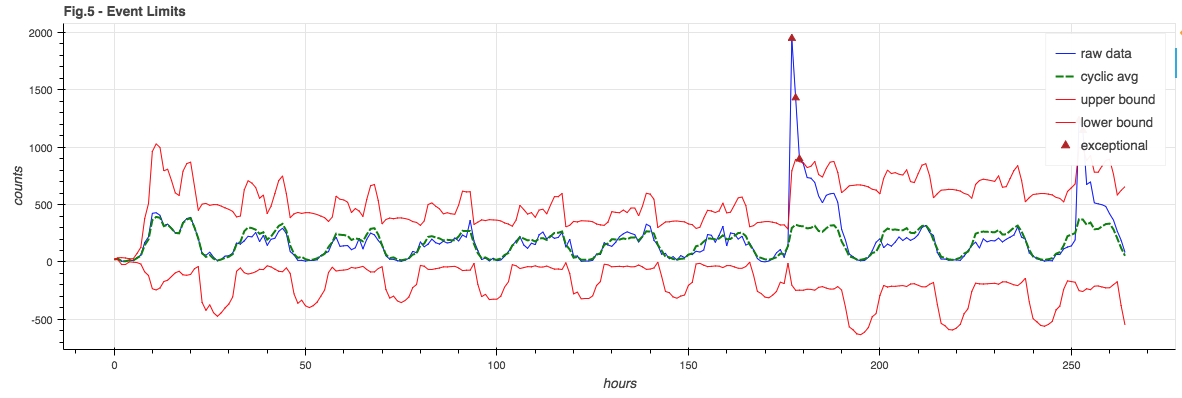
Throwing it all into a pot and mixing, we choose error boundaries that are a combination of the signal model and the sub-cycle standard deviation and note any point where the raw signal exceeds the expected bounds:

Event Floor

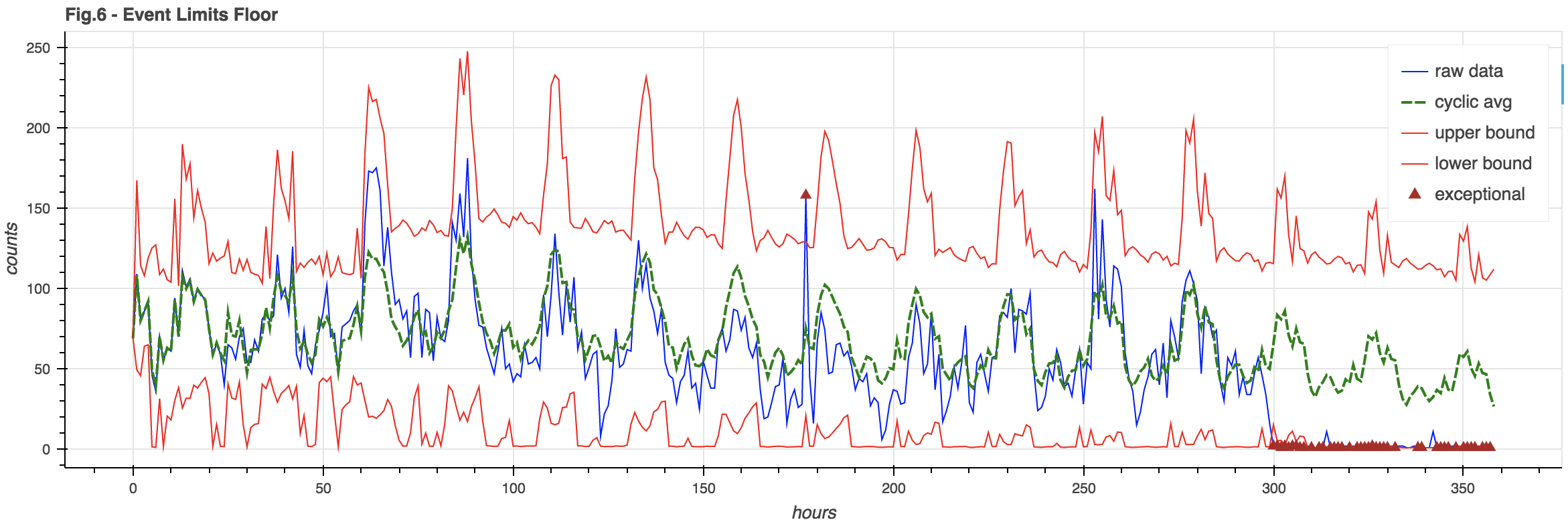
You may note in Figure 5 how the lower bound goes negative.  This is silly – you can’t have negative event counts. Also, for a weak signal where the lower bound tends to be negative, it would be hard to notice when the signal fails completely – as it’s still in bounds.

It can be useful to enforce an event floor so we can detect the failure of a weak signal. This floor is arbitrarily chosen to be 3% of the cyclic model (though it could also be a hard constant):

The End

Playing with data is a ton of fun, so all of the Python code that generated these examples (plus a range of sample data) can be found in GitHub here:

https://github.com/bazaarvoice/event_monitor_test

References

For your reading pleasure:

[1] Automatic Anomaly Detection in the Cloud Via Statistical Learning

[2] STL: A Seasonal-Trend Decomposition Procedure Based on Loess